Earth Observation on a Budget: Finding Solar Farms with a 42k-Parameter Model

Solar farms are expanding rapidly across the UK, but keeping track of where they are, and when they appeared, isn't straightforward. In this post, we'll map them using satellite imagery and a surprisingly small neural network with only ~42k parameters.

We're going to do this using the Tessera foundation model, a pre-trained AI model that already understands satellite imagery in a similar way to how Large Language Models 'understand' text. Using Tessera is a little different from a Large Language Model in that you don't interact with the model directly but rather use pre-generated embeddings for the areas you want to analyse. These embeddings are available at 10m resolution and form a rich summary of that point on Earth's light and radar reflectance over a calendar year, its temporal-spectral characteristics.

We actually used Tessera when we went hunting brambles a few months back. In that instance, we created a pixel-wise model to predict whether a specific 10-meter square contained brambles. This is very easy to do with the efficient sampling support in Geotessera and works fine when the entity is defined purely by its surface temporal-spectral characteristics. But what if the entity you are looking for is defined by its shape and surroundings? For example, a single pixel might be asphalt but whether it is part of a car park or a road must take into consideration its surroundings. In this post we're going to classify solar farms, which exhibit this property. Despite having similar spectral characteristics what separates a solar farm pixel from a rooftop solar install is the size and shape of the solar panels around them.

We could simply classify whether a 1km tile contains a solar farm. However, it's usually more useful to map the exact shape of the farm pixel-by-pixel. This technique is called semantic segmentation, a specific type of dense prediction.

So step one, we need to find some solar farms. For this we use two data sources: OpenStreetMap and the UK government's Renewable Energy Planning Database. We join the OSM solar farm polygons with the REPD to find farms that have an operational date in REPD or a start date in OSM before 2024, this helps filter out farms built in 2024 or 2025. We want to find solar farms that existed throughout 2024.

Now we have a set of solar farm polygons, we need to divide this into train, validation and test sets. For this we use a 25km checkerboard split with roughly 78%, 11% and 11% train, validation and test respectively. We split this way to avoid leaking data from partial and neighbouring polygons. This results in 760 train polygons, 112 validation and 118 test.

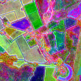
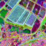
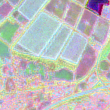
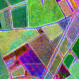
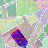
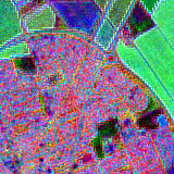
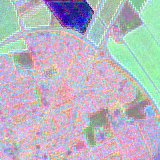
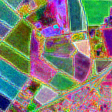
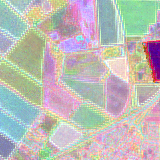
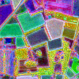
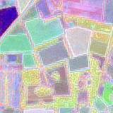
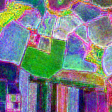
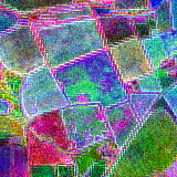
We then produce a set of tiles around each polygon, each 160x160 (so 1.6km x 1.6km). As the Tessera embedding is 128 dimensions, this effectively gives us 128 channel images. Here are a couple with just the first 3 channels of the Tessera embeddings.

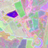
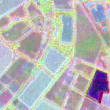
For training targets, we have a binary true/false for each pixel in the image depending on whether it is contained within a solar farm polygon or not.

Now we have these tiles we can train a model using them. For this we use a Convolutional Neural Network (CNN), specifically a UNet. This network design has an encoder-bottleneck-decoder structure with skip connections between the stages and crucially lets us do dense prediction, that is, gives us a prediction at every point. We use a nano-sized UNet configuration, which is only ~42k parameters. It may seem surprising to use such a small model but we've found the richness of Tessera's embeddings means we often don't need very large models. Smaller models mean fewer parameters to fit and in general, less training data. They're also much faster to train, this nano-sized model can be trained in about 15 minutes on CPU alone.

To train the model we use a combination of the Dice loss and the Binary Cross Entropy (BCE) loss. The Dice loss encourages the model to overlap the predicted solar farm regions with our ground-truth regions whilst BCE penalises the model pixel-by-pixel for being wrong, this survey paper has a list of all the possible losses one could use and their properties. We also apply label smoothing (a technique that makes the model less confident in its predictions), which helps it tolerate labelling errors, the kind we probably have through our assumptions about the negatives surrounding solar farms as well as any missing solar farms in OSM that might be in our training tiles.

A final trick is that we 'stretch' our training data through augmentations: random cropping, flipping, and rotating the tiles. This forces the model to learn the essential features of solar farms rather than memorising specific orientations or positions. I was concerned that the orientation of solar panels was actually a strong signal and the rotational and flip augmentations would be harmful but they seem to give a small benefit instead.

Training this takes less than 4 minutes on a Ryzen 9950X + NVIDIA RTX 5090 machine. I'm fairly sure this could go faster with a bit more optimisation. To evaluate the model we focus on the Intersection-over-Union (IoU) which measures the overlap between the model's prediction and the ground truth and divides this by their combined union. The trained model reaches 0.76 IoU on the evaluation set, with a precision of 0.80 and recall of 0.93, which isn't bad at all for a model where we've had to make some strong assumptions around our training data.

Now we have a small trained model, we can use it to do inference. I've run the model over 2017-2024 in the UK. Here's some animations showing growth of solar farms (many of these existed before 2017) in Cornwall and Devon:

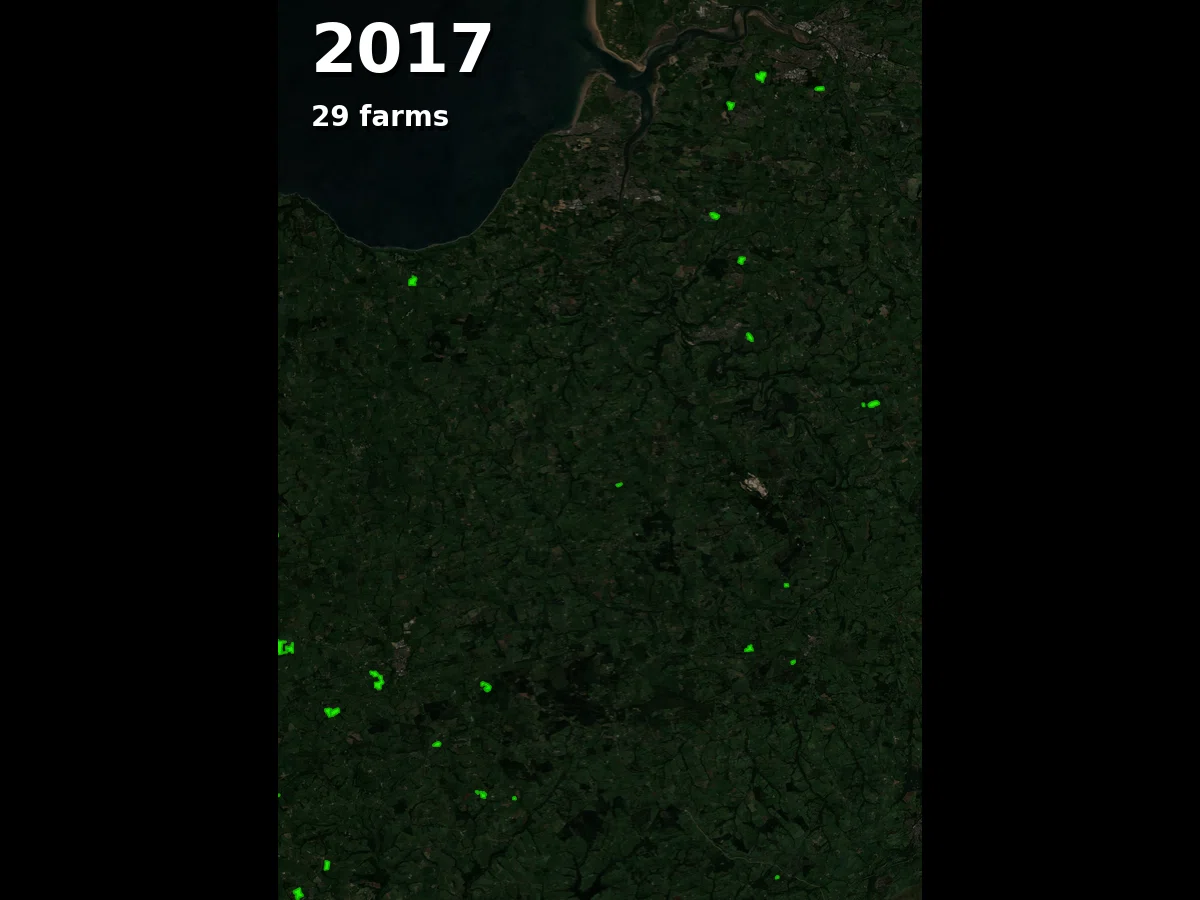
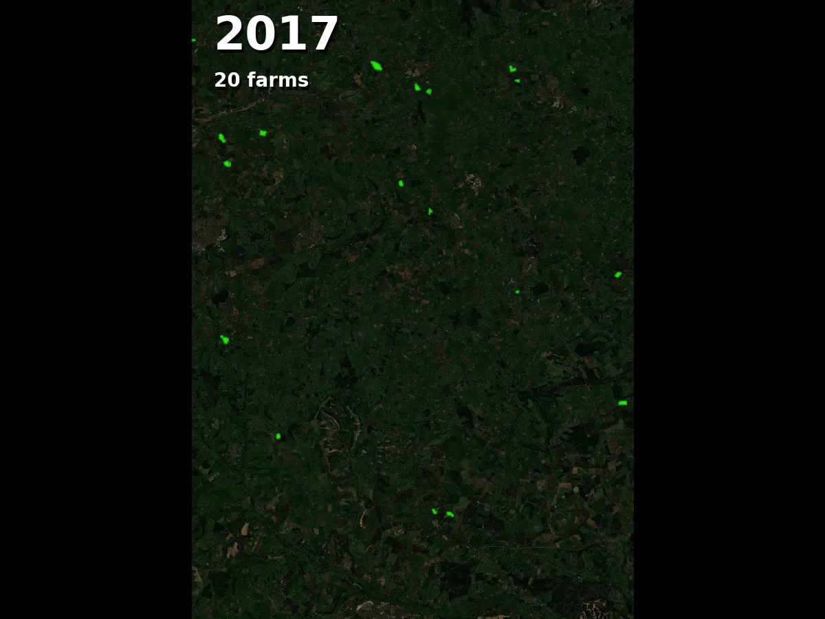
(Both of the above use cloudfree composites from https://s2maps.eu by EOX IT Services GmbH which contains modified Copernicus Sentinel data 2017-2024)

Here's a picture of a chunk of England and Wales, the black areas are solar farms the model identified:

Note: You can also download the model-generated geojson for the whole of the UK, though this has not been validated and almost certainly contains some level of false positives.

Lastly, inferring tiles that are not in the train/validation/test set has revealed a few detected solar farms that don't seem to be in OSM. Determining that is tricky from Sentinel 2 alone, once we have access to a higher resolution source of imagery we should submit the missing ones.

This demonstrates that effective Earth observation doesn't necessarily require massive compute resources. By leveraging the rich, compressed information in Tessera's embeddings, we were able to train a model with only ~42k parameters to identify solar farms across the UK.

There's a general recipe here for using Tessera to detect almost anything that's visible from space:

1. Get your Ground Truth: Start with a dataset of polygons for the thing you want to find. We used OpenStreetMap and the REPD, but you could use any GIS database or even hand-label a small region.
2. Split Spatially: Don't just split your data randomly into train/validation/test sets. Use a spatial split (like our 25km checkerboard) to ensure your model learns to generalize rather than just memorizing the landscape. This is especially important when you are doing classification in very dense areas and where entities can end up very close to each other.
3. Start with the smallest model you can, it may surprise you: As we saw in our solar farm example, even a ~42k parameter model produced good results. As we found in our Tessera paper even linear models performed reasonably. This makes inference very cheap, when inferring over large landscapes you may find your bottleneck is actually bandwidth.

Give it a go and let me know what you find.