Teaching Bloom Filters new tricks

I've had a few interesting conversations around text indexing recently with friends and something that's fallen out is that there are some really cool data structures you build that are extensions of Bloom filters. The techniques for constructing them don't seem to be that widely known so this blog post intends to remedy that.

We will start by examining a variant of the traditional Bloom filter and then we'll look at ways we can generalise the model to produce new types of probabilistic data structures and understand what properties they might have.

Bloom Filters

To begin with, let's take a look at what a Bloom filter is and how it works so we're all on the same page.

Loosely a Bloom filter is a data structure into which you can add a set of elements. Later you can query it with any of those elements and it will return true. Crucially it might also return true for elements that weren't in the set with some (tunable) probability. The benefit you get from this trade-off is that Bloom filters can be very compact.

Trade-offs

How big this benefit is depends on two things. First, how high a probability of an incorrect answer (a false positive) your application can tolerate and second, how large the items are in the set you want to track.

For the first case, let's look at a simple example. Imagine if you were a social network and you want to maintain a cache of your most active ten million users. Each user has is identified by a 32-bit integer. If we naively stored the identifiers of our most active million users we're need 320 million bits or 40 megabytes. On the other hand, if we're willing to accept a 1% false positive rate then a Bloom filter needs just over 11 megabytes. A decent win.

The benefits become much greater as soon as you have large keys. As we'll see in a minute this is because Bloom filters use hashing to avoid storing the keys themselves. If instead of 32-bit user identifiers we are storing urls which could be 320 bits upwards then the win becomes significantly greater. Storing ten million is suddenly >400 megabytes but a bloom filter still clocks in at 11 megabytes for a 1% false positive rate or 17 megabytes for a 0.1% false positive rate.

False positives

Bloom filters are suited to situations where they can filter out the need to do some work and where a false positive just means some wasted work. A good example would be a local Bloom filter sitting in front of a remote key-value cache. The filter can contain the set of keys the remote cache holds the values for and can filter out needless network requests for keys that aren't present. A false positive in this case means we end up doing a request to the remote cache when not necessary.

How they work

Let's look at how a Bloom filter actually works. For those already familiar with Bloom filters, for presentation purposes we're only going to discuss Partitioned Bloom filters as this makes the mathematics simpler and exact.

A Bloom filter consists of an array of \(m\) bits \(B\) and \(k\) hash functions \(h_0..h_{k-1}\). The hash functions take a key \(x\) and map it to a location in \(B\). The hash functions are assumed to be independent of each other. That is if we hash some value "foo" with \(h_0\) then the result should give us no information about the result from hashing with \(h_1\).

Adding to a filter

To add to the Bloom filter we hash the key with the hash functions and use their results to set bits in the array \(B\). More specifically:

for i = 0 to k-1
    j = h[i](x)
    B[i*k+j] = true

Each hash function indexes into a subrange of size \(\frac{m}{k}\) i.e if there are 4 hash functions and array \(B\) is 256 bits then the first hash function picks a position in 0 to 63, the second hash function 64 to 127 and so on. These are later referred to as a hash function's partition.

Querying a filter

To check a Bloom filter for an element we again use the hash functions to hash the key (resulting in the same positions we would have had if we had added the element) and check the array positions they generate in \(B\). Again, some some pseudo code:

p = true /* whether the element is present or not */
for i = 0 to k-1
    j = h[i](x)
    p = p & B[i*k+j]
return p

Why they work

Let's reason out how this works. If we have the element "foo" and add it to a Bloom filter, it will result in a number (\(k\)) of positions in the array \(B\) being set to true. If we then test that same Bloom filter with "foo" we check those same positions and if they are all true then we probably added "foo" at some point in the past to the filter. There can never be a false negative, if we added "foo" those bits must have been set.

There can however be false positives, we may have added some other keys which just so happened to generate positions that covered all the ones that "foo" would hash to. This is the source of false positives in Bloom filters. We can actually calculate the probability that this will occur.

False positive probability for k=1

To simplify let us have a Bloom filter with a single hash function (so \(k=1\)) and with array \(B\) of size \(m\) bits.

A single element is added with the routine we specified above. What is the probability that a bit in \(B\) is set? Since \(h_{0}\) can pick any position¹ then the probability that a bit is set is \(\frac{1}{m}\).

Now comes testing. We test the single element we added. The position will be the same as when we added it, so we'll correctly return that it is present. What if we tested a different element to the one we just added to the Bloom filter? What is the probability that we get a false positive? For a false positive to occur the element we are testing must map to a position that was already set in the array \(B\). We've already calculated that as \(\frac{1}{m}\).

Now instead of a single element, let us consider what happens if we add \(n\) elements and then test something not in those elements.

For each element we add, the probability that a bit position won't be set is \(1-\frac{1}{m}\). After adding \(n\) elements, the probability the bit hasn't been set is \((1 - \frac{1}{m})^n\).

Testing an element that wasn't one we added, we want to know the probability that the bit has been set by one of the previous \(n\) elements. This is complement of the event that it hasn't been set previously, so:

An intuitive way of looking at this is that it is the percentage of 1s set in \(B\) after we add \(n\) items. To test out our simple filter, if the size of \(B\) (\(m\)) is 512 bits and we add 32 elements then the false positive rate if we test a new element that wasn't in the original set is:

So about 6.1%. If we add another 32 elements this increases to 11.8% and so on.

Generalising to multiple hash functions

How do we extend this to multiple hash functions? For partitioned Bloom filters we don't need to deal with collisions between hash functions e.g where \(h_0("foo")\) and \(h_1("foo")\) give the same result. To reiterate, a false positive is where all bit positions in \(B\) for an element tested, but not initially added, are set.

Let's add a second hash function to our simple filter. Now we have \(h_0\) and \(h_1\). To get a false positive we would have needed the bit in \(h_0\)'s partition to be set and the bit in \(h_1\)'s partition. The probability that a bit is set in the 0th partition when an element is added is \(\frac{1}{\frac{m}{2}} = \frac{2}{m}\) because each partition is now \(m/2\) in size as there are two) That the bit is not set after \(n\) elements are added is \((1 - \frac{2}{m})^n\). For the two (independent) hash functions we end up with:

This generalises to:

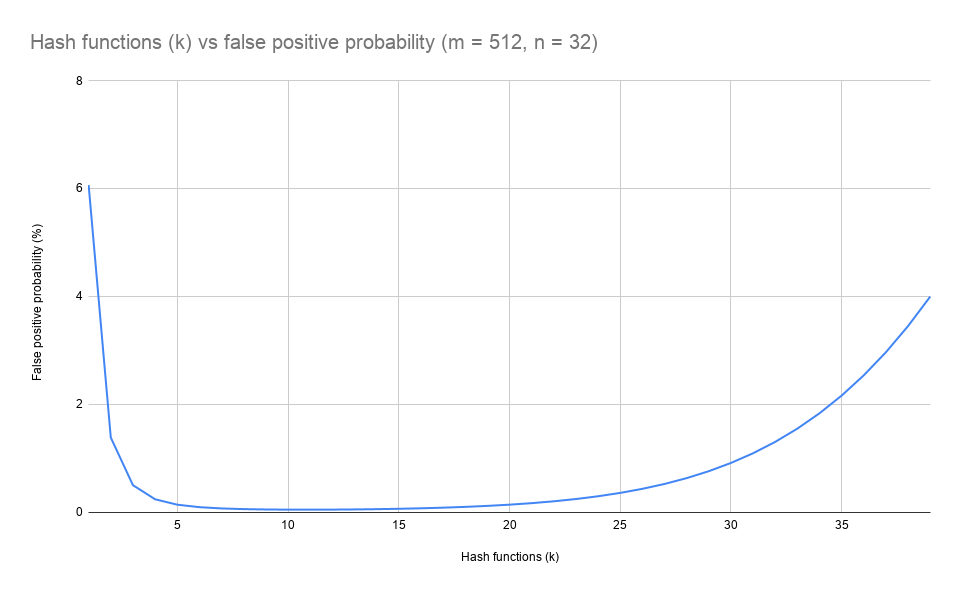
We can quickly work our earlier example again. If B is 512 bits (\(m = 512\)), have 4 hash functions (\(k = 4\)) and we add 32 elements (\(n = 32\)) then we end up with:

Which is 0.2%. Increasing k initially reduces the false positive rate but there's an optimum number (\(k_{opt}\)) before the rate starts to rise. In this example that is \(k = 11\):

Generalising Bloom filters

Now we understand how a Bloom filter works, let's look at how we can generalise the technique and apply it to create some data structures with interesting properties. We'll start by sketching out a general structure and then look at how traditional Bloom filters fit within it.

For the generalised data structure we have an array \(B\) as before but instead of bits we have state of type \(T\) i.e \(B[0]\) is data of type T at the first position in array \(B\).

To add to the generalised Bloom filter we have an input element \(x\) and associated data \(y\). We use \(k\) hash functions (\(h_0\), \(h_1\), etc..) as before. The algorithm is:

for i = 0 to k-1
    j = h[i](x)
    B[i*k+j] = combine(B[i*k+j], y)

So the main difference from before is that we use the combine function and element's associated data to update the state at the hash partition location.

Now let's look at how we would query the generalised Bloom filter:

p = list() /* empty list */

for i = 0 to k-1
    j = h[i](x)
    p.append(B[i*k+j])

return reduce(p)

Here we take the state each hash partition location, make a list of them and pass them to a reduce function. The reduce function returns a result that is some value \(d\) or none.

Lastly we're going to state that the result from querying our generalised Bloom filter will have a one-sided error. We define a third function error and say that if an element \(x\) with associated data \(y\) is added to the generalised Bloom filter then querying for element \(x\), will always contain some value \(d\) and the function error(\(y\), \(d\)) will always return true. If an element \(x\) with associated data \(y\) was not added to the filter then querying will return none or with some (tunable) probability a value \(d\) which error(\(y\), \(d\)) could return true or false for.

So to summarise, our parameters are a type \(T\) for the data array and three functions combine, reduce and error. It turns out that if we pick those four parameters carefully, we can maintain a one-sided error. We'll start with the traditional Bloom filter and then get more adventurous.

Fitting the traditional filter

\(T\) in the traditional filter is a single bit. combine is the max function², reduce is the min function and error is equals.

We also need to modify the input slightly, \(x\) is still the element to be added but the associated data \(y\) is 1 if the element is in the set we added to the filter and 0 if it is not.

If you plug these in to the earlier pieces of pseudo code you should be able to convince yourself that the filter performs identically to the standard description of a partitioned Bloom filter.

Maxmin-based Bloom filters

It turns out if we leave combine as the max function, reduce as the min function and error is \(d \geq y\) then we can still get one-sided errors as long as the elements of type T have a total order.

By a total order we mean that we can compare any two elements of type T³. We'll see later why we're being very specific about this.

Here's an example filter that would satisfy the above requirements. Assuming the associated data \(y\) for each element is a positive integer (think files with a corresponding sizes in kilobytes) then we could use a maxmin-based Bloom filter with T being an unsigned integer. We initialise all elements of \(B\) to 0 and don't allow 0 as a \(y\).

To add to the example maxmin filter:

for i = 0 to k-1
    j = h[i](x)
    B[i*k+j] = max(B[i*k+j], y)

And to query:

p = list() /* empty list */

for i = 0 to k-1
    j = h[i](x)
    p.append(B[i*k+j])

return min(*p) /* min in list */

For an \(x\) added to the example filter, a query returns a result greater than or equal to the associated data \(y\) seen with \(x\). For \(x\) that wasn't added to the filter we will return none or with some probability, a random number from the filter.

There's actually two types of error here:

1. We test an element \(x\) that we haven't added to the Bloom filter and get a value back for it instead of none. We call this a false positive.
2. We test an element \(x\) that we have added to the Bloom filter and get a value back that is higher than the associated value \(y\) we originally added.

Let's start with the false positive probability. We can reuse most of the reasoning from the partitioned Bloom filter false positive derivation earlier. Instead of the bit in \(B\) having been set by a different \(x\) we're instead interested in the element in \(B\) being greater than zero, which means it has been set before.

Since we have \(m\) elements in \(B\), the probability that an element is set to greater than zero on adding to the filter is still \(\frac{1}{m}\). After \(n\) additions the probability that it is still zero is \((1 - \frac{1}{m})^n\). So we again have the same probability of giving a false positive as the traditional case:

What about the second error? For this to happen each of the \(k\) hash partition locations for an element \(x\) must contain a value that is higher than the associated data \(y\). They all must because we take the minimum. There's a bit of difficulty involved in calculating this directly since this kind of error requires a hash collision in each partition and for that collision to result in a higher resulting value. The probability clearly depends on \(y\), if \(y\) is very low (or even the minimum we could see, which is 1) then any collision may lead to this error. If \(y\) is the maximum we could see then no collision will lead to this error.

For now let us go with a very pessimistic assumption that a collision results in a higher value, implying \(y\) is the minimum we will see. This gives us an upper bound on the probability of the second type of error.

Assume we add \(x\) to the filter and we now add a second item. Again we start with a single hash function \(k = 1\) and element array \(B\) of size \(m\). What is the probability there was a collision? We picked a location randomly (using \(h_0(x)\)) for our element \(x\) and now we're picking one again for the second one - the probability of picking the same one is \(\frac{1}{m}\).

Now we add \(n\) items, what's the chance we didn't collide? Not colliding after one is \(1-\frac{1}{m}\). After \(n\) items we end up with \((1-\frac{1}{m})^n\). Similar to earlier on with the traditional Bloom filter but reversed, an intuitive way of looking at this is the percentage of unset elements in \(B\).

So for a single hash function, our estimate (\(d\)) for the associated data \(y\) is exact with probability at least \((1-\frac{1}{m})^n\). Specifically:

What is the situation with multiple hash functions? As we are taking the min then we only need one of the partitions not to have a collision to get an exact answer e.g not where there has been a collision in every partition.

The probability of having a at least one collision in a partition after \(n\) elements is:

for \(k\) partitions this is:

Which is the same as the equation we worked out for the first class of error! If we step back though this should make intuitive sense. Both class of error depend on the proportion of data elements that are non-zero in \(B\). In the first class of error we might read all non-zero elements and incorrectly return a value instead of none and in the second class of error the more set elements we have the greater the chance we have of colliding in every partition.

I should point out at this point that this is a very pessimistic bound. It assumes that any collision leads to an increase in the stored value. There's also a question we've skirted around in this discussion and that is if we make an error of the second class, how big is our over-estimate? I think there's a follow-up blog post on that - though at this stage I'm not sure we can make statements on the over-estimate without making assumptions as to the distribution of \(y\). I may be wrong, let's discuss on twitter: tweet me.

Another thing to note about this filter is that while we only specified it for elements \(x\) with accompanying data \(y\), you can add \(x\) multiple times to the filter with different \(y\)s and the filter will return an estimate for the maximum \(y\) it encountered.

Generalising this model further

Just to recap. For Maxmin filters we have combine as the max function, reduce as the min function and error is \(d \geq y\). Our elements are of type T and have a total order.

We can go further than this with a technique Boldi & Vigna showed in 2004 called Compressed Approximators.

For Compressed Approximators we have combine as the least upper bound, reduce as the greatest lower bound and error is still \(d \geq y\). We'll define these terms in a second. The elements are of type T and form a lattice. For T, this means two things.

First, it means we have some way of comparing two elements of type T, a partial order. The partial part means not all elements are comparable - this is contrast to a total order, where all elements are.

The second is that for any two elements of type T we can find:

1. the smallest element of type T that is greater than or equal to those two elements (the least upper bound)
2. the largest element of type T that is less than or equal to those two elements (the greatest lower bound)

This is convenient because we need to be able to do those two things for combine and reduce.

We'll look at an example now to try to build up an intuitive feeling of what's going on. We base our example around the inclusion order of sets, which is a partial order⁴. Inclusion order means that if all elements of A are also in B i.e A is a subset of B (\(A \subseteq B\)) then \(A \leq B\). For inclusion order, the least upper bound of two sets is their union and the greatest lower bound is their intersection⁵.

A multi-member Bloom Filter

Armed with this lattice, let's turn to a practical application. Imagine you have assets with a key \(x\) that may be cached on one or more of multiple caching servers all of which are infront of some authoritative source (an origin for a CDN, for example). The caching servers may be ephemeral and so we don't want to simply rely on hashing the key to a single server.

The most naive option would be to maintain a Bloom filter for each of the servers but this requires us to potentially do as many tests as we have servers. We can construct a Compressed Approximator for this problem which we only need to test once.

To add to the multi-member Bloom filter we do the following, assuming \(x\) is our key, \(y\) is the server it is now cached on, \(k\) is the number of hashes and \(B\) is an array of sets.

for i = 0 to k-1
    j = h[i](x)
    B[i*k+j] = B[i*k+j].add(y)

So for each hash function and partition, we simply add \(y\) to the set at the hash's index. Assuming add adds to the set if it exists or if not, instantiates it to the singleton set containing just the parameter.

To query the filter we do:

p = set() /* empty set */

for i = 0 to k-1
    j = h[i](x)
    if i == 0 then
        p = B[i*k+j]
    else
        p = intersection(p, B[i*k+j])

return p

We loop over each hash function and partition, taking the intersection of all the sets at those locations⁶.

Again we have a data structure with two possible types of error. As with the maxmin filter, the first type of error is that we test an element we have not added to the filter and we will mistakenly return a set of servers it may be cached on instead of the empty set.

The second type of error is if we test an element we have added to the filter we may get back a set of caches that contains servers the item is not cached on in addition to the right server.

We can use the derivation from earlier for the first type of error, the probability of a false positive is:

For the second error we can also make a similar argument to the maxmin filter, our probability of getting an extra caching server back is at most that of our false positive rate⁷.

Recap and conclusion

So to recap, we've discussed the standard Bloom filter and derived a probability for the false positive rate of the partitioned variant. We then looked at maxmin Bloom filters which generalise them to elements that have a total order, including deriving probabilities for the false positive rate and the event that the value the filter returns is higher than the original value added. Finally we looked at a further generalisation for elements that have a partial order, Compact Approximators, and looked at one specific data structure using that model.

We should be able to use this knowledge to come up with other novel probabilistic data structures based on Bloom filters that have properties which make them better suited to practical problems. I have a whole laundry list of other ones to write up for the next holiday. Want to stay tuned? Follow me on twitter: @sadiqj